
Warning: this document is still work in progress. Feel free to send comments but do not consider it final material.
The idea behind error diffusion is to compute the error caused by thresholding a given pixel and propagate it to neighbour pixels, in order to compensate for the average intensity loss or gain. It is based upon the assumption that a slightly out-of-place pixel causes little visual harm.
The error is computed by simply substracting the source value and the destination value. Destination value can be chosen by many means but does not impact the image a lot with most methods in comparison to the crucial choice of error distribution coefficients.
This is the simplest error diffusion method. It thresholds the image to 0.5 and propagates 100% of the error to the next (right) pixel. It is quite impressive given its simplicity but causes important visual artifacts:
![]()
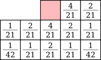
The most famous error diffusion method is the Floyd-Steinberg algorithm [5]. It propagates the error to more than one adjacent pixels using the following coefficients:
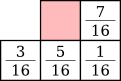
The result of this algorithm is rather impressive even compared to the best ordered dither results we could achieve:

![]()
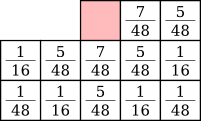
Jarvis, Judice and Ninke dithering [7] (sometimes nicknamed JaJuNi) was published almost at the same time as Floyd-Steinberg. It uses a much more complex error diffusion matrix:

![]()
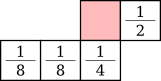
Zhigang Fan came up with several Floyd-Steinberg derivatives. Fan dithering [8] just moves one coefficient around:


![]()
Shiau-Fan dithering use a family of matrices supposed to reduce the apparition of artifacts usually seen with Floyd-Steinberg:

![]()
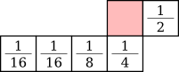

![]()
By the way, these matrices are covered by Shiau’s and Fan’s U.S. patent 5353127.
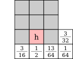
Stucki dithering [6] is a slight variation of Jarvis-Judice-Ninke dithering:

![]()
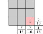
Burkes dithering is yet another variation [10] which improves on Stucki dithering by removing a line and making the error coefficients fractions of powers of two:

![]()
Frankie Sierra [11] came up with a few error diffusion matrices: Sierra dithering is a variation of Jarvis that is slightly faster because it propagates to fewer pixels, Two-row Sierra is a simplified version thereof, and Filter Lite is one of the simplest Floyd-Steinberg derivatives:


![]()

![]()


![]()
Atkinson dithering [12] only propagates 75% of the error, leading to a loss of contrast around very dark and very light areas (also called highlights and shadows), but better contrast in the midtones. The original Macintosh software HyperScan used this dithering algorithm, still considered superior to other Floyd-Steinberg derivatives by many Mac zealots:


![]()
While image parsing order does not matter with ordered dithering, it can actually be crucial with error diffusion. The reason is that once a pixel has been processed, standard error diffusion methods do not go back.
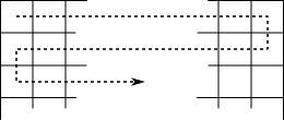
The usual way to parse an image is one pixel after the other, following their order in memory. When reaching the end of a line, we automatically jump to the beginning of the next line. Error diffusion methods using this parsing order are called raster error diffusion:
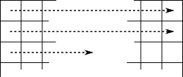
Changing the parsing order can help prevent the apparition of artifacts in error diffusion algorithms. This is serpentine parsing, where every odd line is parsed in reverse order (right to left):
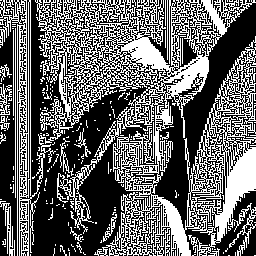
The major problem with Floyd-Steinberg is the worm artifacts it creates. Here is an example of an image made of grey 0.9 dithered with standard Floyd-Steinberg and with serpentine Floyd-Steinberg [13 pp.266—267]. Most of the worm artifacts have disappeared or were highly reduced:
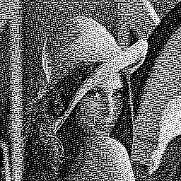
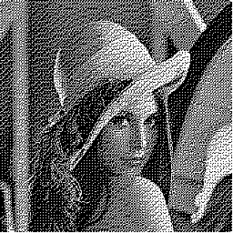
And here are the results of serpentine Floyd-Steinberg on Lena. Only a very close look will show the differences with standard Floyd-Steinberg, but a few of the artifacts did disappear:

![]()
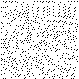
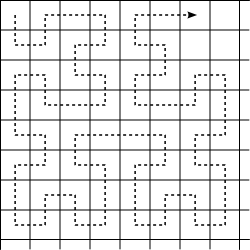
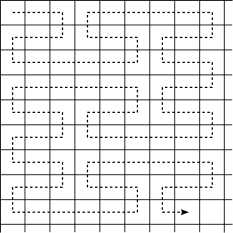
Riemersma dithering [26] parses the image following a plane-filling Hilbert curve and only propagates the error of the last q pixels, weighting it with an exponential rule. The method is interesting and inventive, unfortunately the results are disappointing: structural artifacts are worse than with other error diffusion methods (shown here with q = 16 and r = 16):

![]()
A variation of Riemersma dithering uses a Hilbert 2 curve, giving slightly better results but still causing random artifacts here and there:

![]()
An inherent problem with plane-filling curves is that distances on the curve do not mean anything in image space. Riemersma dithering distributes error to pixels according to their distance on the curve rather than their distance in the image.
We introduce spatial Hilbert dithering that addresses this issue by distributing the error according to spatial coordinates. We also get rid of the r parameter, choosing to distribute 100% of the error.
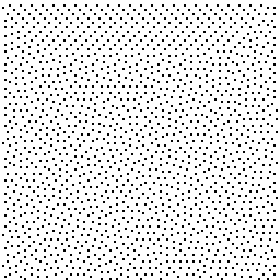
This is spatial Hilbert dithering on a Hilbert curve and on a Hilbert 2 curve. The results show a clear improvement over the original Riemersma algorithm, with far less noise and smoother low-gradient areas:

![]()

![]()
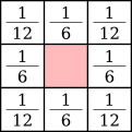
Dot diffusion [14] is an error diffusion method by Donald E. Knuth that uses tileable matrices just like ordered dithering, except that the cell value order is taken into account for error propagation. Diagonal cells get half as much error as directly adjacent cells:
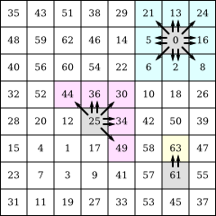
For instance, in the following example, cell 25’s error is propagated to cells 44, 36, 30, 34 and 49. Given the diagonal cells rule, cells 44, 30 and 49 each get 1/7 of the error and cells 36 and 34 each get 2/7 of the error. Similarly, cell 63 gets 100% of cell 61’s error.

![]()
The initial result is not extraordinary. But Knuth suggests applying a sharpen filter to the original image before applying dot diffusion. He also introduces a zeta value to deal with the size of laser printer dots, pretty similar to what we’ll see later as gamma correction. The following two images had a sharpening value of 0.9 applied to them. The image on the right shows zeta = 0.2:

![]()

![]()
Do not get fooled by Knuth’s apparent good results. They specifically target dot printers and do not give terribly good results on a computer screen. Actually, a sharpening filter makes just any dithering method look better, even basic Floyd-Steinberg dithering (shown here with a sharpening value of 0.9, too):

![]()
Dot diffusion was reinvented 14 years later by Arney, Anderson and Ganawan without even citing Knuth. They call their method omni-directional error diffusion. Instead of using a clustered dot matrix like Knuth recommends for dot diffusion, they use a dispersed dot matrix, which gives far better results on a computer display. This is a 16×12 portion of that matrix:

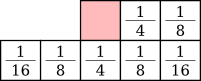
The preferred implementation of omni-directional error diffusion uses a slightly different propagation matrix, where top and bottom neighbours get more error than the others:

![]()
Small error diffusion matrices usually cause artifacts to appear because the error is not propagated in enough directions. At the same time, such matrices also reduce the sharpened aspect common in error diffusion techniques.
Ostromoukhov suggests error diffusion values that vary according to the input value. The list of 256 discrete value triplets for d1, d2 and d3 he provides [1] give pretty good results with serpentine parsing:
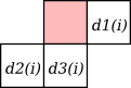

![]()
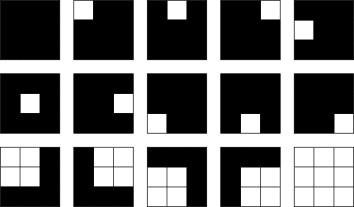
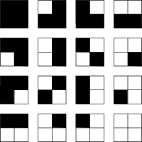
Sometimes, due to physical restrictions of the target media, output is limited to some combinations of pixel blocks, such as the ones shown below:

It is still possible to dither the image, by doing it 4 pixels at a time and simply choosing the block from the list that minimises the global error within the 2×2 block:
![]()
Damera-Venkata and Evans introduce block error diffusion [23], which reuses traditional error diffusion methods such as Floyd-Steinberg but applies the same error value to all pixels of a given block. Only one error value is propagated, a+b+c+d, which is the global error within the block:
⊗
 =
=

Here are the results using the previous pixel blocks:

![]()
Carefully chosen blocks create constraints on the final picture that may be of artistic interest:

![]()
Using all possible pixel blocks is not equivalent to dithering the image pixel by pixel. This is due to both the block-choosing method, which only minimises the difference of mean values within blocks intead of the sum of local distances, and to the inefficient matrix coefficients, which propagate the error beyond immediate neighbours, causing the image to look sharpened.
This example shows standard block Floyd-Steinberg using all possible 2×2 blocks:

![]()
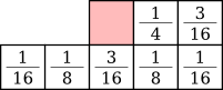
The results on the vertical gradient indicate poor block-choosing. In order to improve it, we introduce a modified, weighted intra-block error distribution matrix, still based on the original Floyd-Steinberg matrix:
⊗
 =
=

The result still looks sharpened, but shows considerably less noise:
![]()
We introduce sub-block error diffusion, a novel technique improving on block error diffusion. It addresses the following observations:
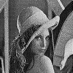
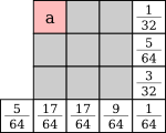
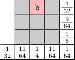
We use m⋅n error diffusion matrices, one for each of the current block’s pixels. Here are four error diffusion matrices for 2×2 blocks, generated from the standard Floyd-Steinberg matrix:


The results are far better than with the original block error diffusion method. On the left, sub-block error diffusion with all possible 2×2 blocks. On the right, sub-block error diffusion restricted to the tiles seen in 3.5:

![]()

![]()
Similar error diffusion matrices can be generated for 3×3 blocks:


Here are the results with all the possible 3×3 blocks, and with the artistic 3×3 blocks seen in 3.5:
![]()

![]()