<?php header("Content-Type: text/html; charset=utf-8"); ?>
<!DOCTYPE html PUBLIC "-//W3C//DTD XHTML 1.1//EN"
       "http://www.w3.org/TR/xhtml1/DTD/xhtml11.dtd">

<html xmlns="http://www.w3.org/1999/xhtml" xml:lang="en">

<head>
   <meta http-equiv="Content-Type" content="text/html; charset=utf-8" />
   <meta name="GENERATOR" content="vim" />
   <meta name="Author" content="sam@zoy.org (Sam Hocevar)" />
   <meta name="Description" content="Libcaca study - 2. Halftoning" />
   <meta name="Keywords" content="libcaca, ASCII, ASCII ART, console, text mode, ncurses, slang, AAlib, dithering, thresholding" />
   <title>Libcaca study - 2. Halftoning</title>
   <link rel="icon" type="image/x-icon" href="/favicon.ico" />
   <link rel="shortcut icon" type="image/x-icon" href="/favicon.ico" />
   <link rel="stylesheet" type="text/css" href="/main.css" />
</head>

<body>

<?php include($_SERVER["DOCUMENT_ROOT"]."/header.inc"); ?>

<p> <span style="color: #aa0000; font-weight: bold;">Warning</span>: this
document is still work in progress. Feel free to send comments but do not
consider it final material. </p>

<div style="float: left;">
   <a href="part1.html">Colour quantisation &lt;&lt;&lt;</a>
</div>
<div style="float: right;">
   <a href="part3.html">&gt;&gt;&gt; Error diffusion</a>
</div>
<div style="text-align: center;">
   <a href="index.html">^^^ Index</a>
</div>

<h2> 2. Halftoning </h2>

<h3> 2.1. Halftoning patterns </h3>

<p> Observe the following patterns. From a certain distance or assuming small
enough pixels, they look like shades of grey despite being made of only black
and white pixels: </p>

<p style="text-align: center;">
  <img src="out/pat2-1-1.png" width="320" height="80"
       class="inline" alt="50% pattern" />
</p>

<p> We can do even better using additional patterns such as these 25% and
75% halftone patterns: </p>

<p style="text-align: center;">
  <img src="out/pat2-1-2.png" width="320" height="80"
       class="inline" alt="25% and 75% patterns" />
</p>

<p> This looks promising. Let’s try immediately on Lena: we will use the
5-colour thresholding picture and replace the 0.25, 0.5 and 0.75 grey values
with the above patterns: </p>

<p style="text-align: center;">
  <img src="out/lena2-1-1.png" width="256" height="256"
       class="inline" alt="25%, 50% and 75% halftoning" />
  <img src="out/grad2-1-1.png" width="32" height="256"
       class="inline" alt="25%, 50% and 75% halftoning gradient" />
</p>

<p> Not bad for a start. But there is a lot to improve.
By the way, this technique is covered by Apple’s <a
href="http://www.freepatentsonline.com/5761347.html">U.S. patent 5761347</a>
[15]. </p>

<h3> 2.2. Screen artifacts </h3>

<p> If your screen’s quality is not very good, you might experience slightly
different shades of grey for the following patterns, despite being made of 50%
black and 50% white pixels: </p>

<p style="text-align: center;">
  <img src="out/pat2-2-1.png" width="240" height="80"
       class="inline" alt="screen imperfections" />
</p>

<p> Obviously the middle pattern looks far better to the human eye on a
computer screen. Optimising patterns so that they look good to the human
eye and don't create artifacts is a crucial element of a dithering
algorithm. Here is another example of two patterns that approximate to
the same shade of grey but may look slightly different from a distance: </p>

<p style="text-align: center;">
  <img src="out/pat2-2-2.png" width="320" height="80"
       class="inline" alt="two different 25% patterns" />
</p>

<h3> 2.3. Ordered dithering </h3>

<p> A generalisation of the dithering technique we just saw that uses a
certain family of patterns is called <b>ordered dithering</b>. It is based on
a <b>dither matrix</b> such as the following one: </p>

<p style="text-align: center;">
  <img src="fig2-3-1.png" width="80" height="80" alt="2×2 dither matrix" />
</p>

<p> Using the matrix coefficients as threshold values yield the following
results for black, white and three shades of grey (0.25, 0.5 and 0.75): </p>

<p style="text-align: center;">
  <img src="fig2-3-5.png" width="507" height="173"
       alt="results of 2×2 dither matrix" />
</p>

<p> The dither matrix is therefore repeated all over the image. The first pixel
will be thresholded with a value of 0.2, the second pixel with a value of 0.8,
then the third pixel with a value of 0.2 again, and so on, resulting in an image
very similar to the one previously seen in 2.1: </p>

<p style="text-align: center;">
  <img src="fig2-3-1b.png" width="240" height="160"
       class="matrix" alt="tiled dither matrix" />
  <img src="out/lena2-3-0.png" width="256" height="256"
       class="inline" alt="2×2 Bayer dithering" />
  <img src="out/grad2-3-0.png" width="32" height="256"
       class="inline" alt="2×2 Bayer dithering gradient" />
</p>

<p> For better readability, the matrix is rewritten as following. The dither
coefficients are trivially computed from the matrix cells and the matrix size:
</p>

<p style="text-align: center;">
  <img src="fig2-3-1c.png" width="297" height="80"
       alt="normalised 2×2 dither matrix" />
</p>

<p> Different matrices can give very different results. This is a 4×4 <b>Bayer
ordered dither matrix</b> [17], recursively created from the previous 2×2
dither matrix: </p>

<p style="text-align: center;">
  <img src="out/fig2-3-2.png" width="161" height="161"
       class="matrix" alt="4×4 Bayer matrix" />
  <img src="out/lena2-3-1.png" width="256" height="256"
       class="inline" alt="4×4 Bayer dithering" />
  <img src="out/grad2-3-1.png" width="32" height="256"
       class="inline" alt="4×4 Bayer dithering gradient" />
</p>

<p> This is an 8×8 Bayer matrix, recursively created from the 4×4 version: </p>

<p style="text-align: center;">
  <img src="out/fig2-3-2b.png" width="240" height="240"
       class="matrix" alt="4×4 Bayer matrix" />
  <img src="out/lena2-3-1b.png" width="256" height="256"
       class="inline" alt="4×4 Bayer dithering" />
  <img src="out/grad2-3-1b.png" width="32" height="256"
       class="inline" alt="4×4 Bayer dithering gradient" />
</p>

<p> This 4×4 <b>cluster dot matrix</b> creates dot patterns: </p>

<p style="text-align: center;">
  <img src="out/fig2-3-3.png" width="161" height="161"
       class="matrix" alt="4×4 cluster dot matrix" />
  <img src="out/lena2-3-2.png" width="256" height="256"
       class="inline" alt="4×4 cluster dot dithering" />
  <img src="out/grad2-3-2.png" width="32" height="256"
       class="inline" alt="4×4 cluster dot dithering gradient" />
</p>

<p> This 8×8 cluster dot matrix mimics the halftoning techniques used by
newspapers: </p>

<p style="text-align: center;">
  <img src="out/fig2-3-3b.png" width="240" height="240"
       class="matrix" alt="4×4 cluster dot matrix" />
  <img src="out/lena2-3-2b.png" width="256" height="256"
       class="inline" alt="4×4 cluster dot dithering" />
  <img src="out/grad2-3-2b.png" width="32" height="256"
       class="inline" alt="4×4 cluster dot dithering gradient" />
</p>

<p> This unusual 5×3 matrix creates artistic vertical line artifacts: </p>

<p style="text-align: center;">
  <img src="out/fig2-3-4.png" width="201" height="121"
       class="matrix" alt="4×4 cluster dot matrix" />
  <img src="out/lena2-3-3.png" width="256" height="256"
       class="inline" alt="4×4 cluster dot dithering" />
  <img src="out/grad2-3-3.png" width="32" height="256"
       class="inline" alt="4×4 cluster dot dithering gradient" />
</p>

<p> There are two major issues with ordered dithering. First, important
<b>visual artifacts</b> may appear. Even Bayer ordered dithering causes
weird cross-hatch pattern artifacts on some images. Second, dithering
matrices do not depend on the original image and thus <b>do not take input
data into account</b>: high frequency features in the image are often missed
and, in some cases, cause even worse artifacts. </p>

<h3> 2.4. Random ordered dithering </h3>

<p> Random dithering can help reduce the major problem caused by halftoning,
which is the apparition of pattern artifacts. The method is as simple as
<b>slightly perturbating dither matrix coefficients</b> (or pixel values)
during the halftoning step. The difficult part is picking up an adequate
perturbation function: too much perturbation and the result is unrecognisable,
too little and the artifacts stay. </p>

<p> For instance, this is the result of 8×8 Bayer dithering perturbated by a
gaussian distribution (mean 0.0, standard deviation 0.08): </p>

<p style="text-align: center;">
  <img src="out/lena2-4-1.png" width="256" height="256"
       class="inline" alt="4×4 Bayer dithering, gaussian perturbation" />
  <img src="out/grad2-4-1.png" width="32" height="256"
       class="inline" alt="4×4 Bayer dithering, gaussian perturbation gradient" />
</p>

<p> Another way to use random number generators to avoid pattern artifacts is
<b>random dither matrix selection</b> [22]. The image space is no longer tiled
with the same matrix over and over again, but with a random selection from a
list of similar dither matrices. </p>

<p> This example shows random matrix selection from a list of six 3×3 dither
matrices: </p>

<p style="text-align: center;">
  <img src="fig2-4-1.png" width="290" height="190"
       class="matrix" alt="four 3×3 dispersed dot matrices" />
  <img src="out/lena2-4-2.png" width="256" height="256"
       class="inline" alt="random Bayer matrix dithering" />
  <img src="out/grad2-4-2.png" width="32" height="256"
       class="inline" alt="random Bayer matrix dithering gradient" />
</p>

<h3> 2.5. Non-rectangular dither tiles </h3>

<p> Another way to avoid disturbing pattern artifacts is to use non-rectangular
dither tiles. Here are several examples, the first one generating slanted
square patterns, the second one hexagonal patterns, then slanted square
patterns again with a slightly different angle, and hexagonal patterns again.
The artifacts usually seen in Bayer dithering do not appear here:
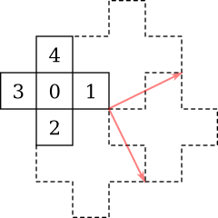
 </p>

<p style="text-align: center;">
  <img src="fig2-5-1.png" width="240" height="240"
       class="matrix" alt="cross dither tile" />
  <img src="out/lena2-5-1.png" width="256" height="256"
       class="inline" alt="cross dithering" />
  <img src="out/grad2-5-1.png" width="32" height="256"
       class="inline" alt="cross dithering gradient" />
</p>

<p style="text-align: center;">
  <img src="fig2-5-2.png" width="270" height="180"
       class="matrix" alt="hex dither tile" />
  <img src="out/lena2-5-2.png" width="256" height="256"
       class="inline" alt="hex dithering" />
  <img src="out/grad2-5-2.png" width="32" height="256"
       class="inline" alt="hex dithering gradient" />
</p>

<p style="text-align: center;">
  <img src="fig2-5-3.png" width="270" height="210"
       class="matrix" alt="square dither tile" />
  <img src="out/lena2-5-3.png" width="256" height="256"
       class="inline" alt="square dithering" />
  <img src="out/grad2-5-3.png" width="32" height="256"
       class="inline" alt="square dithering gradient" />
</p>

<p style="text-align: center;">
  <img src="fig2-5-4.png" width="240" height="210"
       class="matrix" alt="hex2 dither tile" />
  <img src="out/lena2-5-4.png" width="256" height="256"
       class="inline" alt="hex2 dithering" />
  <img src="out/grad2-5-4.png" width="32" height="256"
       class="inline" alt="hex2 dithering gradient" />
</p>

<h3> 2.6. Supercell dithering </h3>

<p> Supercell dithering consists in creating bigger dithering tiles
(supercells) from base tiles. One example is Victor Ostromoukhov’s
<b>CombiScreen</b> method [3]. </p>

<p> 
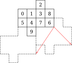
Just like Bayer matrices, non-rectangular tiles can be used to recursively
create bigger patterns, giving finer results. The amount of shades of grey
that can be rendered using a given tile is the number of cells in the tile
plus one. Here are a few examples using tiles seen previously: </p>

<p style="text-align: center;">
  <img src="fig2-6-1.png" width="270" height="240"
       class="matrix" alt="4-wise cross dither tile" />
  <img src="out/lena2-6-1.png" width="256" height="256"
       class="inline" alt="4-wise cross dithering" />
  <img src="out/grad2-6-1.png" width="32" height="256"
       class="inline" alt="4-wise cross dithering gradient" />
</p>

<p style="text-align: center;">
  <img src="fig2-6-2.png" width="270" height="240"
       class="matrix" alt="3-wise hex dither tile" />
  <img src="out/lena2-6-2.png" width="256" height="256"
       class="inline" alt="3-wise hex dithering" />
  <img src="out/grad2-6-2.png" width="32" height="256"
       class="inline" alt="3-wise hex dithering gradient" />
</p>

<p style="text-align: center;">
  <img src="fig2-6-3.png" width="300" height="250"
       class="matrix" alt="4-wise square dither tile" />
  <img src="out/lena2-6-3.png" width="256" height="256"
       class="inline" alt="4-wise square dithering" />
  <img src="out/grad2-6-3.png" width="32" height="256"
       class="inline" alt="4-wise square dithering gradient" />
</p>

<p> 
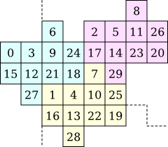
This example shows a tile resembling a Davis-Knuth dragon curve. Though
the tile itself is beautiful, it is in reality only a reorganisation of an
8×8 Bayer dither matrix. Therefore the resulting image is exactly the same
as for classical Bayer dithering: </p>

<p style="text-align: center;">
  <img src="out/fig2-6-4.png" width="325" height="250"
       class="matrix" alt="twin dragon dither tile" />
  <img src="out/lena2-6-4.png" width="256" height="256"
       class="inline" alt="twin dragon dithering" />
  <img src="out/grad2-6-4.png" width="32" height="256"
       class="inline" alt="twin dragon dithering gradient" />
</p>

<p> 
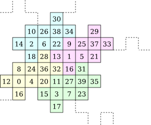
Here are two consecutive iterations of the hexagonal tiling shown
above. Since the area of the original tile is 10 cells, the first iteration
could display 11 different shades of grey. These iterations can display
respectively 31 and 91 shades: </p>

<p style="text-align: center;">
  <img src="fig2-6-5.png" width="240" height="210"
       class="matrix" alt="3-way hex2 dither tile" />
  <img src="out/lena2-6-5.png" width="256" height="256"
       class="inline" alt="3-way hex2 dithering" />
  <img src="out/grad2-6-5.png" width="32" height="256"
       class="inline" alt="3-way hex2 dithering gradient" />
</p>

<p style="text-align: center;">
  <img src="fig2-6-6.png" width="280" height="240"
       class="matrix" alt="9-way hex2 dither tile" />
  <img src="out/lena2-6-6.png" width="256" height="256"
       class="inline" alt="9-way hex2 dithering" />
  <img src="out/grad2-6-6.png" width="32" height="256"
       class="inline" alt="9-way hex2 dithering gradient" />
</p>

<h3> 2.7. Void and cluster method </h3>

<p> Robert A. Ulichney’s <b>void and cluster method</b> [18] is a very generic
method for dither array generation. It mainly targets huge matrices in order
to reduce artifacts caused by tiling. </p>

<p> The process goes through many steps. First, a working pattern matrix
needs to be created: </p>

<ul>
  <li> Generate an empty <i>w×h</i> matrix full of 0s </li>
  <li> Set <i>n</i> cells to 1 </li>
  <li> The working matrix is uniformly distributed:
    <ul>
      <li> Find the 1 with the most neighbours set to 1 and set that cell
           to 0 </li>
      <li> Find the 0 with the fewest neighbours set to 1 and set that cell
           to 1 </li>
      <li> Repeat until the 1 was just put back where it originally was </li>
    </ul>
  </li>
</ul>

<p> Usually <i>n</i> is about 10% of <i>w×h</i>. It can be generated
randomly, loaded from a known pattern, or created using a more powerful
algorithm (chapter 3 will introduce error diffusion algorithms that may be
used to generate the working pattern matrix). </p>

<p> The dither matrix is then generated from the working pattern in three
steps: </p>

<ul>
  <li> Dither indices 0 to <i>n - 1</i> are set using a first copy of the
       working matrix </li>
    <ul>
      <li> <i>n = n - 1</i> </li>
      <li> Find the 1 with the most neighbours set to 1 and set that cell
           to 0 </li>
      <li> In the dither matrix, set the corresponding cell to <i>n</i>
      </li>
      <li> Repeat until <i>n = 0</i> </li>
    </ul>
  </li>
  <li> Dither indices <i>n</i> to <i>w×h/2</i> are set using a second copy of
       the working matrix </li>
    <ul>
      <li> Find the 0 with the fewest neighbours set to 1 and set that cell
           to 1 </li>
      <li> In the dither matrix, set the corresponding cell to <i>n</i>
      <li> <i>n = n + 1</i> </li>
      <li> Repeat until <i>n ≥ w×h/2</i> </li>
    </ul>
  </li>
  <li> Dither indices <i>w×h/2</i> to <i>w×h</i> are set using the same copy
       of the working matrix </li>
    <ul>
      <li> Find the 0 with the fewest neighbours set to 1 and set that cell
           to 1 </li>
      <li> In the dither matrix, set the corresponding cell to <i>n</i>
      <li> <i>n = n + 1</i> </li>
      <li> Repeat until <i>n = w×h</i> </li>
    </ul>
  </li>
</ul>

<p> The key part of the algorithm is the choice of the void finder and the
cluster finder for each step. Best results are achieved using <b>Voronoï
tesselation</b> [19] [22], but simpler methods such as <b>gaussian
convolution</b> [21] give decent results, too. </p>

<p> The following two matrices show the results of the algorithm using
randomly generated initial matrices of size respectively 14×14 and 25×25.
The void and cluster finder uses a simple 7×7 gaussian convolution filter.
Gray cells show the initial uniformly distributed matrix: </p>

<p style="text-align: center;">
  <img src="out/fig2-7-1.png" width="350" height="350"
       class="matrix" alt="14×14 void-and-cluster matrix" />
</p>

<p style="text-align: center;">
  <img src="out/fig2-7-2.png" width="500" height="500"
       class="matrix" alt="25×25 void-and-cluster matrix" />
</p>

<p> Dither matrices generated with the void and cluster method give impressive
results. They are pretty close to the best quality that can be achieved
using standard ordered dithering: </p>

<p style="text-align: center;">
  <img src="out/lena2-7-1.png" width="256" height="256"
       class="inline" alt="14×14 void and cluster dithering" />
  <img src="out/grad2-7-1.png" width="32" height="256"
       class="inline" alt="14×14 void and cluster dithering gradient" />
  <img src="out/lena2-7-2.png" width="256" height="256"
       class="inline" alt="25×25 void and cluster dithering" />
  <img src="out/grad2-7-2.png" width="32" height="256"
       class="inline" alt="25×25 void and cluster dithering gradient" />
</p>

<p> This technique is covered by Ulichney’s <a
href="http://www.freepatentsonline.com/5535020.html">U.S. patent 5535020</a>
and the specific implementation we showed is partly covered by Epson’s <a
href="http://www.freepatentsonline.com/6088512.html">U.S. patent 6088512</a>.
</p>

<div style="float: left;">
   <a href="part1.html">Colour quantisation &lt;&lt;&lt;</a>
</div>
<div style="float: right;">
   <a href="part3.html">&gt;&gt;&gt; Error diffusion</a>
</div>
<div style="text-align: center;">
   <a href="index.html">^^^ Index</a>
</div>

<?php $rev = '$Id$';
      include($_SERVER['DOCUMENT_ROOT'].'/footer.inc'); ?>

</body>
</html>